In this post we continue discussing/translating a rigidty result proven in Grognet for magnetic flows.

Introduction

We finish the discussion from last time, picking up at section 5 and finishing with section 7.

Quasi-geodesics and the sphere at infinity

We start with a few definitions (Definition 5.1).

Definition: We define a cord to be a geodesic curve connecting two points. Given a curve \(c\), we say that \(c\) tends to infinity if \(d(c(0),c(t)) \rightarrow \infty\) as \(\mid t \mid \rightarrow \infty.\)

This leads us to a proposition.

Proposition 3.1: Given a simply connected Riemannian manifold \(M\) with pinched sectional curvature \(-k_0^2 \leq K \leq -k_1^2\), if the magnetic field has norm strictly less than \(k_1\) then its orbits are quasi-geodesics.

Grognet does the proof in two steps. First, she shows that the orbits tend to infinity if the uniform norm of the magnetic field is less than \(k_1\) by using a differential equation on the angle formed by the curvature with a geodesic cord. She then shows that the curve remains in a tubular neighborhood of a geodesic.

Proof: We have the following set up:

1) We have a curve \(c(s)\) of class \(C^2\) with speed \(1\). We denote by

\[S(s) := \frac{d c}{ds}(s)\]

its speed vector.

2) We have the geodesic cord \(s \mapsto \gamma_s(s)\) parameterized with speed \(1\) joining \(c(0) = \gamma_s(0)\) and \(c(s) = \gamma_s(l(s))\).

3) An orthonormal basis \((E_0^s(t), \ldots, E_{n-1}^s(t))\) parallel along the geodesic \(\gamma_s\) with \(E_0^s(t) := \frac{\partial}{\partial t} \gamma_s(t).\)

4) The Jacobi field \(J^s(t) := \frac{\partial}{\partial s} \gamma_s(t)\) of the variation of geodesics \(s \mapsto \gamma_s\). Note that \(J^(0) = 0\) and \(J^s \perp E_0^s\) for all \(t\).

5) The angle \(\alpha(t) \in [0,\pi]\) between the vectors \(E_0^s(l(s))\) and \(S(s)\).

With this set up, we have a lemma.

Lemma 5.1: If the norm of the magnetic field along the curve \(c(s)\) is strictly less than \(k_1\), then there exists \(\epsilon > 0\) such that the angle \(\alpha\) satisfies the following:

\(\cos(\alpha(s)) > \epsilon\) for all \(t \in \mathbb{R}\).

Proof of Lemma 5.1:

We start with a series of observations:

\[\frac{dc}{ds}(s) = \frac{dl}{ds}E_0 + J_s(l(s)),\] \[\cos(\alpha(s)) = \left \langle \frac{dc}{ds}, E_0 \right \rangle = \frac{dl}{ds},\] \[\sin(\alpha(s)) = \|J_s(l(s))\|.\]

Taking the derivative, as long as \(\sin(\alpha) \neq 0\), we have

\[\frac{d\alpha}{ds} = \left\langle b E_0, \frac{1}{\|J_s\|} J_s \right\rangle - \left\langle \frac{1}{\|J_s\|}J_s, \frac{D}{dt} J_s \right\rangle.\]

We note that the comparison of Jacobi fields for geodesic flows tells us that as long as \(\sin(\alpha) \neq 0\) we always have the inequality

\[k_1 \leq k_1 \text{coth}(k_1 l(s)) \leq \left\langle \frac{1}{\|J_s\|^2} J_s, \frac{D}{dt} J_s\right\rangle \leq k_0 \text{coth}(k_0 l(s)).\]

The goal is to use the differential equation set up above to control the angle \(\alpha\). Notice that when \(\sin(\alpha) =0\) we get

\[\frac{d\alpha}{ds} \leq \|b\|_\infty - k_1 \sin(\alpha),\]

where as in the prior post we’re using \(b = i \kappa\) as shorthand. Now consider the differential equation

\[\frac{dy}{dx} = C - k \sin(y) \text{ with } k > C > 0 \text{ and } y(0) = 0.\]

The solution is not pleasant. Let

\[P(y) = \frac{\tan(y/2) - k/C}{\sqrt{k^2/C^2 - 1}}.\]

Then we have

\[x = \frac{1}{C \sqrt{k^2/C^2 - 1}} \ln \left( \text{abs}\left( \frac{P(y) - 1}{P(y) + 1} \cdot \frac{P(0) + 1}{P(0) - 1} \right)\right).\]

As \(x\) goes from \(0\) to \(+\infty\) we see that the function goes from \(0\) to

\[2 \arctan \left(\frac{k}{C} - \sqrt{\frac{k^2}{C^2} - 1} \right) < \frac{\pi}{2}.\]

We now use the spirit of Gronwall’s Lemma. The map \(y\) is a solution of the differential equation with \(k = k_1\) and \(\|b\|_\infty < C < k_1\). We define

\[v(s) = y(s) - \alpha(s).\]

Let \(s\) be a positive real number so that \(v(s) = 0\). We have two cases two consider.

1) If \(\alpha(s) = 0\) then \(s = 0\).

2) If \(\alpha(s) \neq 0\), then \(\alpha'(s)\) exists. We get three more cases to consider.

i) We observe we cannot have \(v'(s) \leq 0\), as this contradicts earlier results. Thus we must have \(v'(s) > 0\).

ii) If \(v'(s) > 0\) and there is a point \(\sigma \in (0,s)\)$ so that \(v(\sigma) = 0\), then we can assume \(v'(\sigma) \leq 0\)

iii) If \(v'(s) > 0\) and there is no such point \(\sigma \in (0,s)\) then we can assume it is strictly negative on the interval \((0,s)\) and this leads to a contradiction.

With all of this being said, we see that \(v\) does not vanish over \((0,\infty).\) We can conclude the proof by choosing

\[\epsilon = \cos(\lim_{s\rightarrow \infty}y(s)).\]

With this, we can observe that \(d(c(0), c(s)) \geq \epsilon \cdot s,\) so by definition the curve tends to infinity. We now make another observation in terms of its cords.

Lemma 5.4: Under the assumptions above, the curve remains a uniformly bounded distance from its cords.

Proof: This follows by the following two equations:

1) We have

\[d(c(s_0), \gamma_{s_1}) \leq \int_{s_0}^{s_1} \left\| \frac{d\gamma_s}{ds}(l(s_0)) \right\|ds = \int_{s_0}^{s_1} \|J_s(l(s_0))\|ds.\]

2) We have

\[\|J_s(l(s_0))\| \leq \frac{sh k_1 l(s_0)}{sh k_1l(s)} \cdot \sin(\alpha(s)).\]

A simple calculation from here gives the result.

Finally, Grognet proves the following Lemma.

Lemma 5.5: If the uniform norm of the magnetic field is strictly less than \(k_1\) then there exists a unique geodesic asymptotic to the curve.

Proof: Set \(s_1\) and take \(s_2 > s_1\). The comparison theorem of Jacobi fields ensures that the velocity vector at \(c(s_1)\) of the geodesic joining \(c(s_1)\) and \(c(s_2)\) converges exponentially as we take \(s_2 \rightarrow \infty.\) Let \(c_+\) be the endpoint of the semi-geodesic limit. Fixing \(s_2\) and taking \(s_1 \rightarrow -\infty\), the same argument yields a point \(c_-\). Observe the two points must be different. The curve \(c\) is in a tubular neighborhood of radius

\[\rho = \frac{\sqrt{1-\epsilon^2}}{\epsilon}\]

of the geodesic connecting \(c_-\) to \(c_+\).

Now observe that Lemma 5.3 gives us the first inequality for a quasi-geodesic, and we get

\[d(c(s_1), c(s_2)) \leq s_2 - s_1\]

giving us the second inequality for a quasi-geodesic. This proves Proposition 3.1.

I’ll omit this, but it’s not too hard at this point to prove the following theorem.

Theorem 3.1: On a manifold \(M\) with sectional curvature \(K\) satisfying

\[- k_0^2 \leq K \leq -k_1^2\]

a magnetic field with norm strictly less than \(k_1\) is orbit equivalent to the underlying geodesic flow.

It’s also not too hard to show the following result. We will also omit the proof of this.

Lemma 5.6: If the magnetic flow is without conjugate points and if \(\|b\|_\infty < k_1\), then any two points of the universal covering of the manifold are connected in a given order by a single trajectory of the magnetic flow.

This leads us to our next definition (Definition 5.2).

Definition: If the flow is without conjugate points, we define the boundary at infinity to be the set of equivalence classes of orbits whose parameters remain a bounded distance as time tends to \(+\infty\). In other words, this is the equivalence class of orbits which are all asymptotic.

A broader stability fact for Anosov flows provides us with the following.

Theorem: Any two points on the boundary at infinity are joined by a unique trajectory of an Anosov flow.

Grognet proves this in the case of Anosov magnetic flows (see Proposition 5.1). The usefulness of such a result comes from the fact that we’re going to use it to show that the geodesic curvature of magnetic flows conjugate to the underlying geodesic flow must be \(0\). We define the geodesic curvature now (Definition 7.1).

Definition: Let \(\kappa \in C^0(M, \mathbb{R})\). The curves with geodesic curvature \(\kappa\) are those curves who are solutions with parameterized speed \(1\) to the following second order differential equation:

\[\frac{D}{dt} \frac{dc}{dt} = \kappa(c(t)) i \frac{dc}{dt}(t).\]

Remark: I believe at this point the reason for introducing more language is because Grognet actually considers a broader class of flows when she’s talking about magnetic flows. She starts with the differential equation and mentions that, while you can get a \(2\)-form from her definition, she doesn’t even require the \(2\)-form to be necessarily closed. By studying geodesic curvature, she’s studying the usual magnetic flows that people like Paternain study.

The final bit of information we’ll need is the following definition (Definition 7.3).

Definition: Two flows are said to have the same marked length spectrum if the lengths of orbits in the same free-homotopy class are the same.

We can now formulate the promised rigidty result.

Theorem 7.3: Let \(M\) be an oriented closed surface with endowed Riemannian metric \(g_1\) and magnetic field \(\kappa\) which satisfies \(\|\kappa\|^2 + \|\kappa\|_\infty < k_1^2.\) We suppose that the magnetic flow \((M, g_1, \kappa)\) is conjugate to the geodesic flow \((M, g_2)\), where \(g_2\) satisfies having strictly negative sectional curvature on \(M\) and is without conjugate points. We also assume that \(g_1\) and \(g_2\) have the same volume. If we assume that the conjugation is absolutely continuous, then the function \(\kappa\) is \(0\) and the metrics are isometric.

Remark: The fact assumption that the conjugation is absolutely continuous is unnecessary, as seen in the most recent Grognet paper on the matter.

Sketch of Proof: We skim over Lemma 7.1 which is essentially a Feldman-Ornstein type result (for reference see Wilkinson’s notes). Letting \(h\) denote the conjugation, we can note everything is nice so that we have

\[h_*(\lambda_1) = \lambda_2,\]

where \(\lambda_i\) is the normalized Liouville measure on the unit tangent bundle of the metric \(g_i\). Moving this to a map on the space of orbits, we see that it has constant Jacobian and sends the measurements

\[\sin(\theta_1) d\theta_1 dt_1\]

to the measure

\[\frac{\text{vol}_{g_1}(M)}{\text{vol}_{g_2}(M)} \sin(\theta_2) d\theta_2 dt_2.\]

Let \((x,v) \in T^1M\), and let \(\theta \cdot (x,v) = (x, \theta \cdot v)\), where the action here is just to rotate the vector \(v\) by \(\theta\). Recall how the boundary at infinity was defined earlier. We’ll say two curves have the same terminal point on the boundary at infinity if they are forward asymptotic, and the same origin point on the boundary at infinity if they are backward asymptotic. Now Grogent considers three maps:

\[\xi, \xi_1, \xi_2 : T^1M \rightarrow (0,\pi].\]

We define \(\xi(v) = \theta > 0\), where \(\theta\) is the smallest angle such that the orbit starting at \(v\) and the orbit starting at \(\theta \cdot v\) share an extreme point (meaning the must either be forward or backward asymptotic). Suppose the orbit of \(v\) has endpoints \(v_+, v_-\) on the boundary at infinity. We define \(\xi_1(v) = \theta > 0\) to be the smallest angle where the orbit of \(\theta \cdot v\) has an endpoint coinciding with \(v_+\), while \(\xi_2(v) = \theta > 0\) is the smallest angle where the orbit of \(\theta \cdot v\) has an endpoint coinciding with \(v_-\). Notice that this doesn’t necessarily mean they share orientation. Observe that \(\xi = \min\{\xi_1, \xi_2\}.\) Observe as well that for an Anosov magnetic trajectory \(c(t)\), we have the maps

\[t \mapsto \xi_1(c(t)), \ \ t \mapsto \xi_2(c(t))\]

are both \(C^1\).

Take \(v \in T^1M\). We can apply the conjugacy \(h\) (understood now as a map on the unit tangent bundle, see Wilkinson’s notes) to both \(v\) and \(\theta \cdot v\) to get a new angle \(\theta' := \theta'(v, \theta).\)

Fix a closed orbit \(\gamma : [0,T] \rightarrow M\) for \((M,g_1, \kappa)\). Grognet points out that (viewing things correctly) we can view \(h\) as a homeomorphism on the set \(h(\gamma) \times (0,\pi]\) to the set

\[\{(\gamma(t), \theta) : 0 \leq t \leq T, 0 \leq \theta \leq \xi(\gamma(t))\}.\]

Moreover this send the Liouville measure to the Liouville measure. Thus:

\[\begin{split} \frac{1}{T} \int_0^T (1- \cos(\xi(\gamma(t)))) dt = \frac{1}{T} \int_0^T \int_0^{\xi(\gamma(t))} \sin(\theta) d\theta dt \\ = \frac{1}{T} \int_0^{T} \int_0^\pi \sin(\theta) d\theta dt = 2. \end{split}\]

Thus we get that \(\xi(\gamma(t)) = \pi\) for all \(t\) in the interval \([0,T]\) (since it is a closed orbit, over \(\mathbb{R}\)). Thus if we rotate by \(\pi\), we know it must share an endpoint with \(\gamma(t)\). This tells us that

\[\begin{split} \pi = \xi(\gamma(t)) \leq \min\{\xi_1(\gamma(t)), \xi_2(\gamma(t))\} \leq \max\{\xi_1(\gamma(t)), \xi_2(\gamma(t)) \} \leq \pi. \end{split}\]

Thus we must have \(\xi(\gamma(t)) = \xi_1(\gamma(t)) = \xi_2(\gamma(t)) = \pi.\) That is, the reverse flow shares both terminal endpoints with \(\gamma(t)\), except in reverse order, and this is the first rotated vector which achieves either of these goals.

Examine \((\gamma(t), \dot{\gamma}(t)) \in T_{g_1}^1M\) – it helps to imagine this with regards to the universal cover and the boundary at infinity. For this fixed \(t\), we can look at the orbit \(c_t\) generated by rotating this vector by \(\pi\). In other words, \(c_t\) is the magnetic flow for \((M,g_1, \kappa)\) at the vector \((\gamma(t), - \dot{\gamma}(t))\). Notice apriori these are just two points on this sort of circle – see the following picture.

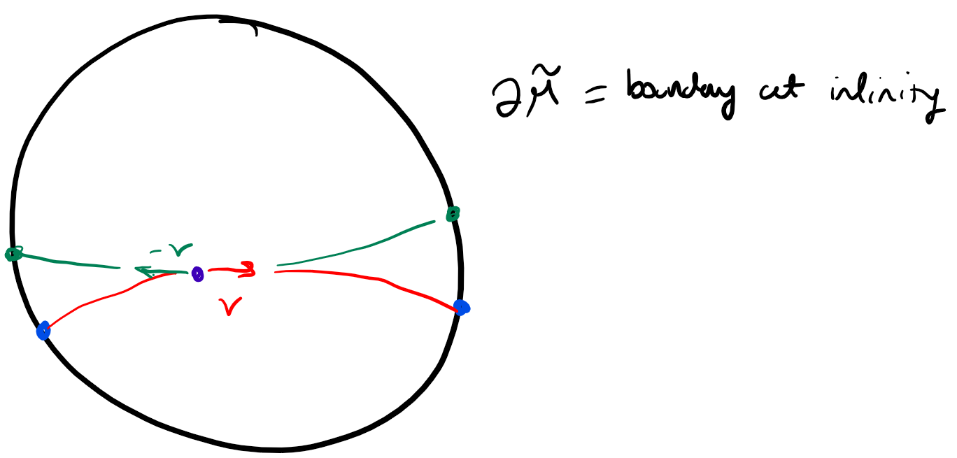
An earlier proposition (Proposition 5.1) ensures that there is a unique curve which joins two points at infinity in a given order. By our above work we have that \(c_t\) share the same endpoints with \(\gamma\) for all \(t\), so they all coincide and are the same curve. This tells us that \(\gamma(t)\) can be “traversed in either direction.” Grognet then claims that this is sufficient for establishing that the geodesic curvature is zero. Let’s assume this fact and see why the rest of the argument follows from this. If we can establish this, then we have established that for every closed orbit, we have \(\kappa \equiv 0\) along it. Since \(\kappa\) is at least continuous and periodic orbits are dense, we get that \(\kappa\) is \(0\) on a dense set. We deduce from here that \(\kappa \equiv 0\), and thus our magnetic flow is just geodesic flow. Now \(h\) is a conjugacy between geodesic flows, and we can invoke Otal’s theorem to finish the result. Thus the metrics are isometric and \(\kappa \equiv 0\), as desired.

We now wish to show that if a closed curve can be traversed in either direction in the sense of above, then it must have geodesic curvature zero. Let’s restrict ourselves to just the closed orbit \(\gamma\) for simplicit, and now we have \(\kappa : \mathbb{R} \rightarrow \mathbb{R}\) a smooth function with

\[\nabla_{\dot{\gamma}(t)} \dot{\gamma}(t) = \kappa(t) i \dot{\gamma}(t).\]

Now traversing it backwards and forwards means that plugging in \(- \dot{\gamma(t)}\) still gives us the same curve, so the same geodesic curvature along that curve. Thus we have

\[\nabla_{-\dot{\gamma}(t)} (-\dot{\gamma}(t)) = \kappa(t) i (-\dot{\gamma}(t)).\]

Using the fact that \(\nabla\) is bilinear, we can simplify this to get

\[-\kappa(t) i \dot{\gamma}(t) = \kappa(t) i \dot{\gamma}(t).\]

This can only happen if \(\kappa(t) = 0.\) Since this is true at each point, we get that \(\kappa \equiv 0\) along the curve, as desired. Thus this establishes Grognet’s conjugacy result.

Remark: Two remarks on the theorem.

1) With results from Croke et al (see Theorem A), we can improve the result to say that the isometry must be isotopic to the identity, not just an isometry.

2) We can actually slightly upgrade the result of the theorem as seen in Grognet’s more recent work (see this paper). In Corollary 10.1 we see that with a few more assumptions on our system we can drop the requirement that \(h\) is absolutely continuous, leading to Theorem 10.2. There are a few more results in that paper which seem to be improvements in the context of a linearized system.