In this post, we discuss a problem from dynamical systems that I’ve been thinking about, as well as the end of Rudin chapter 1.

Personal Life

In real life, my week has mostly been coming back to Columbus Ohio and adjusting to the change. I’ve decided to pick up a little bit of walking, and have been walking around 3 miles a day (most of it in the rain). The rest of my day is essentially devoted to reading Katok and Rudin, and then having meetings discussing what I’ve read, mixing in a little rewatch of Mr. Robot.

Dynamics

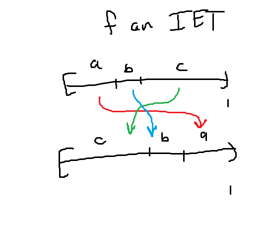
I’ve been really thinking about induced dynamical systems and their relation to the bigger system. In particular, I’ve been stuck on a sequence of problems in Katok. These focus on things called IETs (Interval Exchange Transformations) which are essentially continuous transformations on the interval [0,1] which exchange the order of intervals, usually corresponding to some permutation. The sequence of problems are focused on showing ergodicity of an IET, as seen below.

We recall that for a (finite) measure space \((X, \Sigma, \mu)\) (we will abbreviate it to \((X,\mu)\) since the measurable sets generally come attached to the measure anyhow). A measurable transformation \(T : (X,\mu) \rightarrow (X,\mu)\) is said to be measure preserving if we have that \(\mu(T^{-1}(A)) = \mu(A)\). Note the fact that this is a preimage, rather than the image. The reason for this is that, in general, the image of a measurable map need not be measurable – consider the Borel \(\sigma\)-algbera, and the fact that a continuous map need not have continuous image (though I guess in this case the image could still be measurable, but you get the idea).

An easy example of a measure preserving transformation is the doubling map \(E_2 : S^1 \rightarrow S^1\) define by \(E_2(x) = 2x \pmod{1}\), where we implicitly take the measure to be the Lebesgue measure, viewing \(S^1 = [0,1]/\sim\). One easy exercise is that it suffices to show measure preserving on the generators of a \(\sigma\)-algbera – to see why, notice that preimages play nicely with unions. Using this result, we can take an interval \((a,b) \subset S^1\) and look at its preimage. This will turn out to be the disjoint union of two intervals whose length add up the the length of the original interval. The Lebesgue measure for intervals is just length, so we see that this map preserves the measure of open intervals (and actually preserves the measure of all intervals), so it is a measure preserving map.

Ergodicity, then, is a notion which corresponds to “mixing well”. Implicitly, we’ll assume that our transformation is measure preserving. If we were to independently try to derive the definition of ergodicity, we would essentially want it to say that, given a sufficient amount of time, we want the map to (up to almost everywhere equivalence) hit every measurable set equally well.

To formally define things, we consider a probability measure (so a measure such that \(\mu(X) = 1\)). A map \(T : (X,\mu) \rightarrow (X,\mu)\) which is measure preserving is ergodic if \(T^{-1}(A) \subset A\) implies that \(\mu(A) = 0 \text{ or } 1\). The doubling map (which is a special case of an expanding map) is an example of an ergodic transformation.

Generally it’s not too easy to play with the usual definition of ergodic, so on probability measure spaces we develop a result which gives us a few equivalences. One nice one is that a map \(T : (X,\mu) \rightarrow (X,\mu)\) is ergodic if and only if for all square integrable \(f : X \rightarrow \mathbb{C}\), \(f \circ T = f\) almost everywhere implies f is constant almost everywhere. The backward direction here is easy, since being a probability measure space implies that all measurable sets have finite measure, hence they’re characteristic functions are square integrable and so we get ergodicity by noting that a characteristic function is constant almost everywhere if and only if it is 1 or 0 almost everywhere, and then we integrate. The forward direction, while still relatively easy, is the more interesting direction. There, we do a sort of Fubini/Tonelli argument (if you’ve read the proof in Folland’s “Real Analysis”). You establish that the result holds for characteristic functions, then it holds for simple functions by linearity, then it holds for positive functions by the monotone convergence theorem, then it holds for all functions by linearity and breaking up the function into its positive and negative parts. Note that this sort of method also proves a more general result, which is replacing square integrable with just integrable functions.

The advantage of thinking about square integrable functions over just integrable functions is that we have a Hilbert space, so we can do Fourier tricks to prove ergodicity. We then take some arbitrary square integrable function, write it in terms of its Fourier series (which it must be equal to almost everywhere), and then we compose with T and write that function in terms of its Fourier series, and note that the Fourier coefficients are equal. From there, we generally implement a Riemann-Lebesgue argument (since we have that infinitely many of the coefficients are equal), which forces all but the 0th coefficient to be 0 and so we have that it’s constant almost everywhere, or we have some nice relation which forces whatever condition we are looking for (for example, see linear flows on the torus and rational independence).

In some sense, we have some nice algorithmic strategy for checking ergodicity with this (sometimes we need to get a little tricky, but it’s usually not that tricky). However, in trying to prove that this IET is ergodic, we don’t have the usual tricks in place, so Fourier tricks won’t be helpful here. I’m unsure how to go about it from here, but it’s something that will at least be in the back of my mind.

You can induce the IET by looking at a rotation on a circle and looking at the induced dynamical system on a subinterval. If you label the endpoints of the second interval \(\alpha, \beta\) you have that you can scale the interval by \(1/(1+\beta-\alpha)\) to get a sub interval, and then consider the dynamical system induced on the subinterval \([0, 1/(1+\beta-\alpha)]\) via rotating by \((1-\alpha)/(1+\beta-\alpha)\). It takes a little bit of calculation to show that the induced system will correspond to the IET, and so you have a unique correspondence of all IETs in this form to induced dynamical systems on this subinterval by this rotation. As pointed out to me, showing minimality of this induced dynamical system reduces (thanks to the niceness of \(S^1\)) to looking at the minimality of the whole dynamical system on the circle. This is due to the fact that you can look at the orbit of points on the whole circle, and then the corresponding orbit on the induced system is found by just cutting off the end.

By a known result, minimality of the whole system occurs when the rotation is irrational, so when \((1-\alpha)/(1+\beta-\alpha)\) is irrational. So we get that the IET is minimal iff \((1-\alpha)/(1+\beta-\alpha)\) is irrational, which is at least some condition. Katok implies that it should correspond to \(\beta/(1+\beta-\alpha)\) is irrational, which I don’t quite see yet. He also goes on to imply that minimality (in this case) should correspond to unique ergodicity, but I don’t know these definitions yet so I can’t make any definitive statements. I will hopefully explore this more in the future.

Functional Analysis

It’s still mostly building terminology right now. A lot of the past week has been focusing on seminorms and the topology they generate. A seminorm is essentially just a norm without the positive definiteness property. Hence, a seminorm \(\rho : X \rightarrow \mathbb{R}_{\geq 0}\) is a map which satisfies the triangle inequality, i.e. \(\rho(x+y) \leq \rho(x) + \rho(y)\) for all \(x, y \in X\), and it satisfies a homogeneity property, i.e. \(\rho(\alpha x) = \mid \alpha \mid \rho(x)\) for all \(\alpha\) scalars and \(x \in X\). A family of seminorms \(\mathcal{F}\) on a topological vector space \(X\) is said to be separating if, for all \(x \neq 0\) in \(X\), we have that there exists some \(\rho \in \mathcal{F}\) so that \(\rho(x) \neq 0\) as well. In some sense, the family of functions sees the difference between points, even if the individual functions don’t necessarily see the difference.

There are two nice theorems which relate separating seminorms to local convexity – we have that if \(X\) is a locally convex space, then this implies there exists a family of separating seminorms, and if there exists a family of separating seminorms on \(X\) then we can define a topology on \(X\) with the family so that the space is locally convex. This construction using the Minkowski functional.

First, a set \(A \subset X\) is said to be absorbing if for every \(x \in X\), there exists a \(t > 0\) so that \(x \in tA\). The Minkowski functional can be considered as a function from the space of absorbing subsets of \(X\) to the space of seminorms of \(X\), where \(A \mapsto \mu_A\) is defined by

\[\mu_A = \inf\{t > 0 : t^{-1}x \in A\}.\]

We require \(A\) to be absorbing so that this function is finite. An interesting consequence from Rudin is that this Minkowski function is surjective if we restrict to the case of balanced convex absorbing sets instead of just absorbing sets. In other words, every seminorm arises as a Minkowski functional of a balanced convex absorbing set (I believe this is just for separating families of seminorms, but Rudin mentions this as though this is a broader result. This is something to think more about later.)

The way we generate topologies with separating seminorms is by considering the collection of finite intersections of sets of the form

\[V(\rho,n) = \left\{ x \in X : p(x) < \frac{1}{n} \right\}.\]

If the family is separating, then we have that this will give us a convex balanced local base for a topology \(\tau\). This is essentially just the weakest topology so that every \(\rho\) in the family is continuous.

Rudin gives us a way of generating separating seminorms from a convex balanced local base, and then gives us a way of generating a topology from a family of separating seminorms. A natural question to ask if we start with a convex balanced local base for a topology \(\tau\), generate a family of separating seminorms \(\mathcal{F}\), and then generate topology \(\tau_1\) from this family \(\mathcal{F}\), do we have \(\tau_1 = \tau?\) Rudin answers in the affirmative with a cute little argument. Notice that every \(\rho \in \mathcal{F}\) is continuous with respect to the original topology \(\tau\), so this tells us that \(\tau_1 \subset \tau\). To get the other direction, let \(W\) be in the convex balanced local base. Then we have a functional \(\mu_W\), and an associated set

\[W = \{x : \mu_W(x) < 1 \} = V(\mu_W,1).\]

Note that one needs to actually establish these are equivalent. If done so, we have that \(W \in \tau_1\), and since the local base is contained in \(\tau_1\) this implies that \(\tau \subset \tau_1\). Hence, they are equal.

If we get a countable base, we know from the metrization theorem that the space is then metrizable, so we get a metric and an associated topology to that metric. It turns out that we can show that the metric is compatible with the original topology as well, so that the associated topology is the original topology. In other words, this method is the best method you could ask for.

Similar to the metrization theorem, we get some necessary and sufficient conditions for the normability of a space. A topological vector space will be normable (i.e. there exists a norm whose topology is compatible with the original) if and only if the origin has a convex bounded neighborhood. The argument for this isn’t too difficult, but I’d rather not write it out here.

From my limited knowledge of Functinal Analysis, seminorms will be extremely important, so I expect to read/write more on them as I continue on. Next week will hopefully consist of more Baire category stuff, as well as the Banach-Steinhaus theorem and the Hahn-Banach theorem.