In the seventh recitation we covered lengths of curves, and in the eights we covered applications.

Lengths of Curves

Given a function \(f(x)\) on some interval \(a \leq x \leq b\), we wish to approximate the length of the graph of the curve. If \(f(x)\) is a line, this is easy to do using the Pythagorean theorem. For example, say \(f(x) = 2x\) on \(0 \leq x \leq 1\). The length of this curve will be given by

\[\sqrt{(\Delta x)^2 + (\Delta y)^2} = \sqrt{1^2 + 2^2} = \sqrt{5}.\]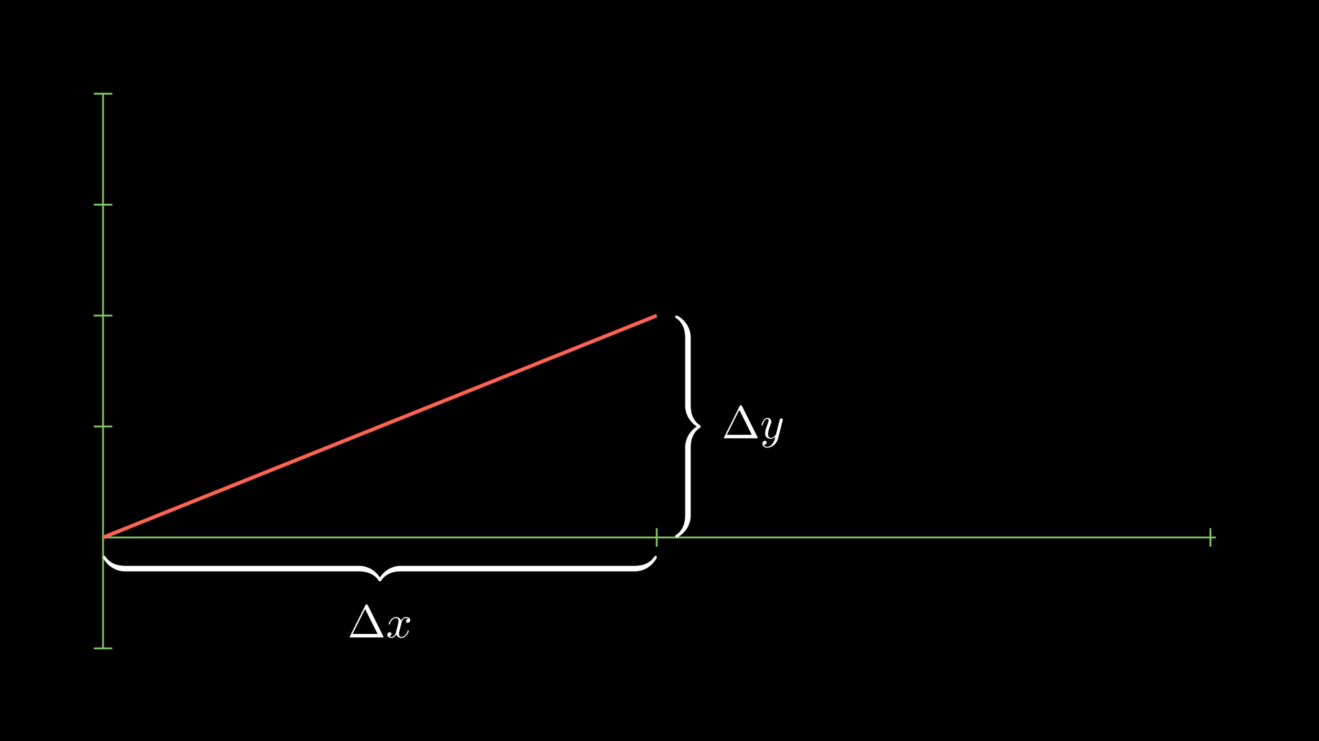

In fact, this works generally as well. If we have a function \(f(x)\), then remembering that \(\Delta x\) means change in \(x\) and \(\Delta y\) means change in \(y\), we can calculate the length of the line connection \(f(x_0)\) to \(f(x_1)\) by using this formula:

\[\sqrt{(\Delta x)^2 + (\Delta y)^2} = \sqrt{(x_1 - x_0)^2 + (f(x_1) - f(x_0))^2}.\]

In the picture below, we do this with \(x_0 = 0\), \(x_1 = 1\), and \(f(x) = x^2\). The blue line is the line connecting these two points.

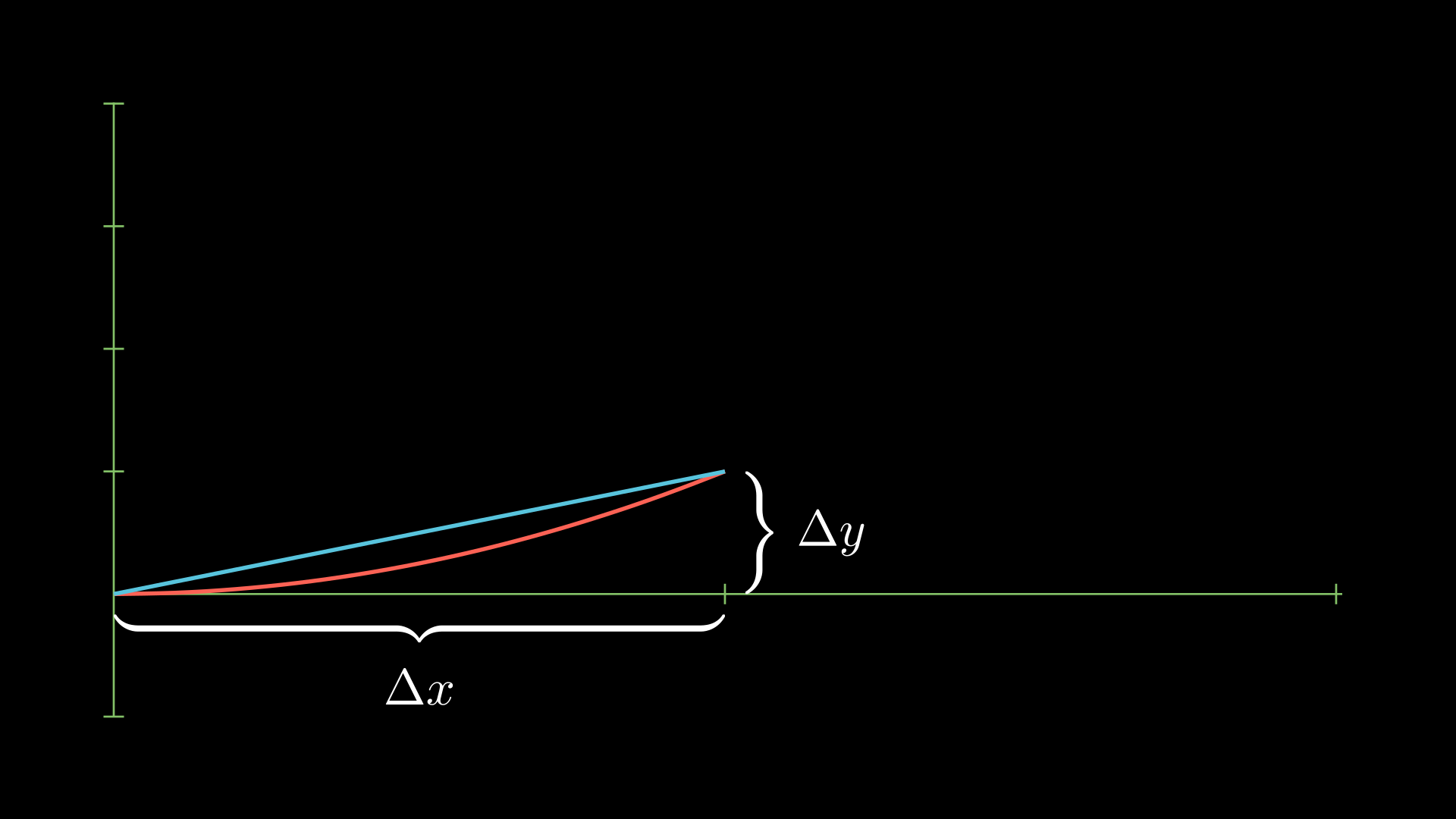
As we let \(x_1\) get arbitrarily close to \(x_0\), \(\Delta x\) gets closer to \(dx\). Similarly, \(f(x_1) - f(x_0)\) gets closer to \(df = f'(x_0)dx\). So we get that the “infinitesmal” length of a curve is given by

\[\sqrt{1 + f'(x_0)^2}dx.\]

Integrating all of the infinitesmal lengths (think of this as adding the lengths) gives us the total length. Thus the arc length of a curve \(y = f(x)\) on the interval \(a \leq x \leq b\) is given by

\[\int_a^b \sqrt{1 + f'(x)^2}dx.\]

Problem: Derive the formula for the circumference of a circle with radius \(r\).

Solution: Remember that “circumference” is a fancy way of saying “perimeter,” so we’re trying to find the length of a curve. A circle is given by the relation

\[x^2 + y^2 = r^2,\]

which if we solve for \(y\) gives

\[y = \pm \sqrt{r^2 - x^2}.\]

Since the shape is symmetric, we can solve for the length of the top part of the circle and then just multiply that by two to get the total length. Step one is to find the derivative of \(y = \sqrt{r^2 - x^2}\). We get

\[y' = -\frac{x}{\sqrt{r^2-x^2}} \implies (y')^2 = \frac{x^2}{r^2-x^2}.\]

We now use our formula:

\[\int_{-r}^r \sqrt{1 + (y')^2}dx = \int_{-r}^r \sqrt{1 + \frac{x^2}{r^2-x^2}}dx = \int_{-r}^r \frac{r}{\sqrt{r^2 - x^2}}dx.\]

Now remember that

\[\frac{d}{dx} \arcsin(x) = \frac{1}{\sqrt{1 - x^2}}.\]

Going back, we can simplify:

\[\frac{r}{\sqrt{r^2 - x^2}} = \frac{r}{r \sqrt{1 - (x/r)^2}} = \frac{1}{\sqrt{1 - (x/r)^2}}.\]

Let \(u = x/r\) so that \(du = dx /r\) or \(r du = dx\). Notice that if \(x = -r\) then \(u = -1\) and if \(x = r\) then \(u = 1\), so

\[\int_{-r}^r \frac{r}{\sqrt{r^2 - x^2}}dx = r \int_{-1}^1 \frac{du}{\sqrt{1 - u^2}} = r \arcsin(u) \Big|_{u=-1}^1.\]

Finally, remember that \(\arcsin(\pm 1) = \pm \pi/2,\) so the length of the top half of a circle is given by \(r \pi\). Since this is half, we multiply it by two to get that the circumference is \(2\pi r\).

Applications of Integrals

There are three formulas we’ll need to remember in this section, but the important part I want to emphasize first is how to derive them. The motivation for this is calculating the area under a curve, so let’s review this quickly.

Area Under a Curve

Suppose we have a continuous function \(f(x)\) on an interval \(a \leq x \leq b\). Remember that we can approximate the area under the curve by using rectangles. There are several strategies we can take here, but for simplicity let’s just always do a “left Riemann sum.” The strategy is to divide the interval up into equal intervals, and then evaluate the function on the left part of the interval. One way of thinking about it is that we’re taking a piecewise defined function which is “piecewise constant” and finding the area of this (which is easy). The hope is that as we take smaller and smaller equal intervals, this gets closer and closer to the real value. To make this precise, let’s do an example.

Take the function \(f(x) = x^2\) on the interval \([0,1]\). Let’s divide it up into ten equal intervals. Notice that the length of each interval must be

\[\Delta x = \frac{\text{Length of total interval}}{\text{Number of intervals}} = \frac{1-0}{10} = \frac{1}{10}.\]

So our intervals look like

\[I_k = \left[ \frac{k-1}{10}, \frac{k}{10} \right] \text{ for } 1 \leq k \leq 10.\]

In order to find the area, we take the left part of each interval (which we denote by \(x_k^*\)) and plug it into the function, and then multiply it with the length of the interval (remember that the area of a rectangle is base times height). So the total area of this piecewise function is

\[\text{Approximate area} = \sum_{k=1}^{10} f \left( x_k^* \right) \Delta x = \frac{1}{10} \sum_{k=1}^{10} \left( \frac{k-1}{10} \right)^2.\]

We can simplify this to get

\[\text{Approximate area} = \frac{1}{10} \sum_{k=1}^{10} \frac{k^2 - 2k + 1}{100},\]

or

\[\text{Approximate area} = \frac{1}{1000} \sum_{k=1}^{10} (k^2 - 2k + 1) = \frac{1}{1000} \left(\sum_{k=1}^{10} k^2 - 2 \sum_{k=1}^{10}k + \sum_{k=1}^{10}1) \right).\]

Next, we need some formulas. Remember that

\[\sum_{k=1}^n k^2 = \frac{n(n+1)(2n+1)}{6}, \sum_{k=1}^n k = \frac{n(n+1)}{2}, \sum_{k=1}^n 1 = n.\]

So

\[\text{Approximate area} = \frac{1}{1000} \left( \frac{10(11)(21)}{6} - 10(11) + 10 \right) = \frac{57}{200}.\]

In fact, we have all of the ingredients to generalize this trick. For \(n\) rectangles, we have that the approximate area is given by

\[\text{Approximate area} = \frac{1}{n^3} \left( \frac{n(n+1)(2n+1)}{6} - n(n+1) + n \right) = \frac{1}{6n^2} - \frac{1}{2n} + \frac{1}{3}.\]

If we take \(n \rightarrow \infty\), we get that the area under the curve should be \(1/3\). This matches what happens if we take the integral as well:

\[\int_0^1 x^2dx = \frac{x^3}{3} \Big|_{x=0}^1 = \frac{1}{3}.\]

Essentially, what is happening is that we really only know how to deal with constant functions, and so we’re breaking the problem up into smaller and smaller constant functions which converges to the answer we want. We’re going to now generalize this idea to calculating mass.

Mass, Work, and Work on a Collection of Particles

If we have constant density, then we know that the mass will be equal to the “volume” times the density (volume here depends on the dimension). If we have variable density, then this does not apply. However, we can use the philosophy of calculus to derive what the mass should be. Suppose the density of a wire is given by a function \(\rho(x)\) and suppose it’s on an interval \(a \leq x \leq b\). We can copy the same idea as last time. If we break up the interval into \(n\) smaller intervals, we can take the left endpoint \(x_k^*\) (or really any point in the interval) and calculate the density on these smaller intervals. These smaller intervals have length \(\Delta x\), so using the fact that mass is volume times density we get

\[\text{Mass of } I_k = \rho(x_k^*) \Delta x.\]

Adding these up will give us the approximate mass:

\[\text{Approximate mass} = \sum_{k=1}^n \rho(x_k^*) \Delta x.\]

If we take a limit as \(n \rightarrow \infty\), this will converge to the actual mass. So by the Riemann sum intuition, we should have

\[\text{Total mass} = \lim_{n \rightarrow \infty}\sum_{k=1}^n \rho(x_k^*) \Delta x = \int_a^b \rho(x)dx.\]

This is our first formula. A similar trick gives us the formula for work when force isn’t constant:

\[\text{Work} = \int_a^b F(x)dx.\]

Finally, we can use the same trick to derive the work done for pumping a liquid out of the top of a tank:

\[\text{Work} = \int_a^b \rho g A(y) D(y) dy,\]

where \(\rho\) is the density, \(g\) is the gravity, \(A(y)\) is the cross-sectional area, and \(D(y)\) is the distance the particles must move.

An Application of the Trick

To finish these notes out, let’s try working through Problem 5 on the handout.

We wish to calculate the amount of blood that passes through a given cross-section of an artery per unit time – this is called “flux.” When the rate \(v\) is constant, the flux \(\Phi\) is easy to calculate:

\[\Phi = A \cdot v,\]

where \(A\) is the area. Generally, things are not constant. If an artery has radius \(R\), then the rate at which blood is passing is given by

\[v(r) = \frac{P}{4 \eta \ell} (R^2 - r^2),\]

where \(r\) is the distance from the center, \(P\) is the pressure difference between the ends of the artery, \(\ell\) is the length of the artery, and \(\eta\) is the viscosity of the blood. Using our trick, let’s find out how to calculate total flux.

Since the rate \(v\) is in terms of the distance from the center, the interval we’ll be looking at is \(0 \leq r \leq R\). What we can do is chop this up into \(n\) smaller intervals of constant length \(\Delta x\). Unlike our earlier calculations, we have this other equation \(A\) we need to worry about. Suppose the endpoints of our interval \(I_k\) is given by \([x_k^*, x_{k+1}^*]\). Remember these are circles, so the area at a given \(r\) is

\[A(r) = \pi r^2.\]

To calculate the area of the region with radii bounded between \([x_k^*, x_{k+1}^*]\), what we’ll need to do is subtract the bigger area from the smaller. We get that the area is given by \(A(x_{k+1}^*) - A(x_k^*).\) Remember from the Riemann sum trick that these two points are going to get closer and closer to each other in the limit. In particular, we can use an approximation here. If \(\Delta x = x_{k+1}^* - x_k^*\), then

\[A'(x_k^*) \Delta x \approx (x_{k+1}^*)^2 - (x_k^*)^2.\]

Thus we can approximate the area by

\[A'(x_k^*) \Delta x = 2 \pi (x_k^*) \Delta x,\]

and we can approximate the flux with

\[\text{Approximate flux} = \sum_{k=1}^n v(x_k^*)2 \pi (x_k^*) \Delta x.\]

As we take \(n \rightarrow \infty\), we can use our Riemann sum intuition to say that

\[\text{Total flux} = \int_0^R 2\pi x v(x)dx.\]

Substituting in the formulas gives us the appropriate integral.